1.1 Systems of Linear Equations 
 1.1 Systems of Linear Equations
 Each Section and Topic title are links. At the end of each section, there is a link back to this table.
- 1.1.1 What is Linear Algebra
- 1.1.2 Systems of Linear Equations
- 1.1.3 Geometry of Linear Systems of Equations
- 1.1.4 Square Linear Systems
- 1.1.5 Rectangular Linear Systems
- 1.1.6 The Row Picture for Linear Equations
- 1.1.7 The Row Picture for Larger Linear Systems
- 1.1.8 Vectors
- 1.1.9 The Column Picture
- Definition: Linear Combination
- Figure 7: Linearly Independent Vectors
- Definition: Consistent and Independent Linear System
- Figure 8: Linearly Dependent Vectors
- Definition: Consistent and Dependent Linear System
- Figure 9: Two Anti-Parallel Vectors
- Definition: Inconsistent and Dependent Linear System
- Example 3 - Circuits
- Figure 10: Two Loop Circuit
- Exercise 6 - Recognizing Dependence
- 1.1.10 Linear Combination and Span
- Video Lecture 5: Span
- Definition: Span
- Figure 11: The Span of One Vector
- Figure 12: The Span of Two Dependent Vectors
- Figure 13: The Span of Two Independent Vectors
- Figure 14: The Span of Three Dependent Vectors
- Figure 15: Two Independent and One Dependent Vector
- Figure 16: The Span of Three Independent Vectors
- Exercise 7 - Spanning Questions in $\mathbb{R}^3$
- 1.1.11 Solving Systems of Linear Equations
- 1.1.12 Exercises
- 1.1.13 True/False Questions
- 1.1.14 Multiple Choice Questions
- 1.1.15 Challenge Exercises
- copyleft
1.1.1 What is Linear Algebra
Definitions Are Important
To begin our study of linear algebra, it is important to have a basic notion of our subject before diving in. Linear algebra is a subject with a lot of interconnected ideas and a rich vocabulary for understanding and communicating these ideas. Let us start with the definition of our course topic.
Definition
Linear Algebra is the mathematical study of Linear Equations
$$ a_1 x_1 + a_2 x_2 + \ldots + a_n x_n = b, $$
Linear Mappings,
$$ \left[ \begin{array}{c} x_1 \\ x_2 \\ \vdots \\ x_n \end{array} \right]\mapsto a_1 x_1 + a_2 x_2 + \ldots + a_n x_n, $$
and their associated representations using vectors and matrices.
However, that isn't terribly helpful until we know more about what those boldface terms mean.
Videos
Throughout these online notes we will see videos to study. These videos are placed at the best point to study them. Videos are often decorated with an icon to make them easy to find in the notes. There are three sources of video for our class.
3Blue1Brown
 3Blue1Brown
by Grant Sanderson features a series videos that explore linear algebra at a high level. These videos demonstrate the primary concepts of this subject in a way that will help you develop your intuition without being bogged down by technical details. The 3Blue1Brown video series is a superb way to develop and reinforce your understanding of the interrelated geometrical and algebraic ideas of linear algebra. Watch these videos several times during your semester.
3Blue1Brown
by Grant Sanderson features a series videos that explore linear algebra at a high level. These videos demonstrate the primary concepts of this subject in a way that will help you develop your intuition without being bogged down by technical details. The 3Blue1Brown video series is a superb way to develop and reinforce your understanding of the interrelated geometrical and algebraic ideas of linear algebra. Watch these videos several times during your semester.
- Watch each video where it appears in the notes prior to reading the textbook or attempting the exercises in WebAssign.
- Watch all covered videos prior to the midterm to help you study for the midterms tests.
- Watch all of them the week before the final exam. You'll be amazed how much all the pieces fit together on those second and third viewings.
A Vision of Linear Algebra
- Professor Gilbert Strang's
 A Vision of Linear Algebra and his course Linear Algebra includes video, downloadable pdf versions of the included slides, lecture notes, sample exams with solutions, recitation videos, and problem sets with solutions. You can download the entire course if you want a personal copy.
Instructor Videos
- There are several videos created by Dr. Nathan Thompson and myself providing lectures, examples, demonstrations and, problem solutions. Instructor videos may be found in these online notes, and in their web-based learning management system (LMS) such as Blackboard.
Every student should study the videos included in the online notes.
- Students enrolled in a Traditional Classroom Instruction (TCI) course should watch these videos before attending the corresponding lecture.
- Students enrolled in an HYB-Online course must realize that these online notes and web-based videos replace their course lectures. Students enrolled in such an online course need to take notes, study the videos, and ask questions online. In this way, an HYB-Online student receives the same level of support as a TCI student.
Everyone should start with Video Lecture 1 featuring Emeritus Professor Gilbert Strang, Five Factorizations of a Matrix.
Video Lecture 1: Five Factorizations of a MatrixThis video is a good place to start and a good place to finish your study of linear algebra. This video will help everyone understand the path of this course, and review for the final exam.
Vocabulary is Important
Finally be aware that this course contains an abundance of vocabulary that normally lower level mathematics courses understate. Vocabulary and concept questions will be the subject of most questions in proctored exams in this course. Every word in the online notes displayed in bold text indicates a vocabulary term. Definitions of important vocabulary introduced by this course are found in Definition boxes.

1.1.2 Systems of Linear Equations
In Chapter 6 we will learn a very formal definition of a linear transformation. For now, we need one that is based on our previous mathematical education to help us get started understanding the structure and importance of linear algebra.
The Essence of Linear Algebra
Video Lecture 2: The Essence of Linear Algebra
This video gives us an introduction into the relationship between the geometrical and computational aspects of linear algebra. We need to master these concepts of linear algebra and let computers perform numerical computations.
- Create mathematical models that describe STEM phenomena,
- Specify the necessary computations to computing devices, and
- Interpret the results.
Linear Expressions
A linear expression is a mathematical expression in which each variable that appears in the expression has only the power one.
| Algebraic Expression | Classification |
|---|---|
| $3x + 2y$ | is a linear expression |
| $5x + 9y^2$ | is not a linear expression because the variable $y$ is raised to the power of 2. |
| $5x + \dfrac{1}{y}$ | is not a linear expression because the variable $y$ is raised to the power -1. |
| $3x + \sin(y)$ | is not a linear expression because $\sin(y) = \displaystyle\sum_{k=0}^{\infty} (-1)^k\dfrac{y^{2k+1}}{(2k+1)!}$ |
Linear Equations
The difference between an expression and an equation is that an equation must have a verb phrase. An equation is a complete mathematical sentence. The phrases "is equal to", " is greater than", " is less than or equal to" are common verb phrases represented by specific symbols. A linear equation has a linear expression on the left-hand side of an equality symbol and another linear expression on the right-hand side.
| Algebraic Equation | Classification |
|---|---|
| $3x + 5y = 2$ | is a linear equation |
| $3x + 5y = 0$ | is a linear equation |
| $3x = -5y$ | is a linear equation |
Generally one wants to arrange linear equations to have a constant on the right-hand side of the equation. One expresses a pattern by using letters to represent our constant real number instead of just examples of specific real numbers. This means that $ax + by = c$ represents a linear equation with variables $x$ and $y$; and constants $a$, $b$ and $c$. We refer to the variables as unknowns and refer to the constants as coefficients. To express three equations with three unknowns, one might write
$$ \begin{array}{rcl} x + y - z & = & 0 \\ -x + y + z & = & 2 \\ 3x - y + z & = & 2 \end{array} $$
Linear Systems
A list of several equations is called a system of equations. This course will be focused on finding solutions to systems of linear equations.
We will not just solve linear systems of equations. We will also analyze them and their mathematical structure so that we gain an understanding of how systems of linear equations can be solved, how they can be utilized in our work, and how best to understand their geometric nature.
To avoid running out of letters for coefficients we will employ subscripts such as $a_{21}$. The subscripts indicate that this coefficient is the coefficient in the second equation for variable number one. This works so well that subscripts are utilized for our variables. We will define our three unknowns to be $x_1$, $x_2$ and $x_3$. Finally, we need to represent the constants on the right-hand sides of the three equations $b_1$, $b_2$ and $b_3$.
$$ \begin{array}{rcl} a_{11}x_1 + a_{12}x_2 + a_{13}x_3 & = & b_1 \\ a_{21}x_1 + a_{22}x_2 + a_{23}x_3 & = & b_2 \\ a_{31}x_1 + a_{32}x_2 + a_{33}x_3 & = & b_3 \end{array} $$
This allows us to talk about all linear systems with three equations and three unknowns. We can discover what geometric properties they share. In this course we will develop a vocabulary for describing linear systems such as this one in addition to discovering algebraic methods to solve them.
Exercise 1 - Rates of Motion
Two planes start from Los Angeles International Airport and fly in opposite directions. The second plane starts 2 hours after the first plane, but its speed is 120 kilometers per hour faster. Five hours after the first plane departs, the planes are $1960$ kilometers apart. Find the airspeed of each plane.
First try this on your own. Use Check Your Work to confirm your answer. If you do not know how to start, scroll the Follow Along block to the bottom of your screen and expand it. Then scroll just enough to see only the first line or two of the argument. Then try again.
Check Your Work
$s_1 = 200$ km/hr and $s_2 = 320$ km/hr.
Follow Along
The unknown values are the air speeds of each plane which we can call $s_1$ and $s_2$ for the speed of planes 1 and 2, respectively. Rate times time equal distance so we have two equations for their distances from the airport which we can call $d_1$ and $d_2$. If the first plane starts at time $t=0$ until time $t=5$, then
$$ \begin{align*} d_1 &= 5s_1 \\ d_2 &= s_2(5-2) \qquad\text{because plane 2 starts two hours later} \\ s_2 &= s_1 + 120 \qquad\text{because plane 2 flies 120 kilometers per hour faster} \\ d_1 + d_2 &= 1960 \end{align*} $$
With a little algebra one obtains
$$ \begin{align*} 5s_1 + 3s_2 = d_1 + d_2 = 1960 \end{align*} $$
We can simplify these equations to get a system of linear equations.
$$ \begin{align*} -s_1 +\,\ s_2 &= 120 \\ 5s_1 + 3s_2 &= 1960 \\ \end{align*} $$
If we multiply both sides of the first equation by -3 and then add the two equations, then we obtain
$$ \begin{align*} 3s_1 - 3s_2 &= -360 \\ 5s_1 + 3s_2 &= 1960 \\ \hline 8s_1 \qquad\ \ &= 1600 \end{align*} $$
Dividing both sides of the resulting equation by $8$, and solving for $s_2$ yields
$$ \begin{align*} s_1 &= 200 \text{ km/hr} \\ s_2 &= 200 + 120 = 320 \text{ km/hr} \end{align*} $$
1.1.3 Geometry of Linear Systems of Equations
The Geometry of Linear Systems
Video Lecture 3: The Geometry of Linear SystemsAs we studied in Dr. Strang's lecture, the geometry of a linear system of equations can be viewed primarily from two different viewpoints called the row picture and the column picture. Both geometrical understandings are necessary to appreciate how linear systems are applied and solved. However the row picture has computational limitations that will become clear in the next few examples. Not only are Multidimensional Hyperplanes difficult to envision, the computational technique of substitution used to solve the linear system according to this view is very inefficient for computational machines and people.
The abstraction of a vector space, the column picture, and linear combinations scale to even the very large systems utilized by modern STEM applications.
1.1.4 Square Linear Systems
Examples
Examples appear throughout the notes to illustrate important ideas and give concrete understanding to new topics.
Consider a system of 8 equations with 8 unknowns.
Example 1 - Small Example
$$ \begin{align*} 3x_1 + 4x_2 -\,\ x_3 + 2x_4 - 2x_5 -\,\ x_6 + 2x_7 + 4x_8 &=\ \ \ 15 \\ 4x_1 + 4x_2 + 4x_3 + 2x_4 - 4x_5 -\,\ x_6 + 2x_7 -\,\ x_8 &=\ \ \ 26 \\ -3x_1 - 3x_2 + 3x_3 + 2x_4 - 4x_5 + 2x_6 - 2x_7 +\,\ x_8 &= -15 \\ 4x_1 + 4x_2 + 4x_3 -\,\ x_4 + 3x_5 + 3x_6 + 2x_7 - 2x_8 &=\ \ \ 15 \\ x_1 + 4x_2 +\,\ x_3 +\,\ x_4 + 2x_5 - 3x_6 +\,\ x_7 + 2x_8 &=\ \ \ 7 \\ -4x_1\qquad\,\ \ - 4x_3 - 3x_4 - 2x_5 \qquad\,\ \ - 3x_7 - 2x_8 &=\,\, -2 \\ -2x_1 + 3x_2 + 3x_3 + 2x_4 + 4x_5 \qquad\,\ \ - 3x_7\qquad\,\ \ &= -16 \\ \qquad\,\ \ - 3x_2 + 4x_3 - 4x_4 - 4x_5 +\,\ x_6\qquad\,\ \ + 2x_8 &=\ \ \ \ 7 \\ \end{align*} $$
We must develop more powerful techniques to solve realistic linear systems of equations than the ones picked up in pre-calculus and calculus education. Most linear systems required by data science, large language models, pattern recognition, and robotics consist of thousands of equations and thousands of unknowns. Some large language models have reached 1 trillion equations and 1 trillion unknowns (parameters). Using subscripts is especially useful for even larger systems of equations.
$$ \begin{array}{rcl} a_{11}x_1 + a_{12}x_2 + a_{13}x_3 + a_{14}x_4 + a_{15}x_5 + a_{16}x_6 + a_{17}x_7 + a_{18}x_8 & = & b_1 \\ a_{21}x_1 + a_{22}x_2 + a_{23}x_3 + a_{24}x_4 + a_{25}x_5 + a_{26}x_6 + a_{27}x_7 + a_{28}x_8 & = & b_2 \\ a_{31}x_1 + a_{32}x_2 + a_{33}x_3 + a_{34}x_4 + a_{35}x_5 + a_{36}x_6 + a_{37}x_7 + a_{38}x_8 & = & b_3 \\ a_{41}x_1 + a_{42}x_2 + a_{43}x_3 + a_{44}x_4 + a_{45}x_5 + a_{46}x_6 + a_{47}x_7 + a_{48}x_8 & = & b_4 \\ a_{51}x_1 + a_{52}x_2 + a_{53}x_3 + a_{54}x_4 + a_{55}x_5 + a_{56}x_6 + a_{57}x_7 + a_{58}x_8 & = & b_5 \\ a_{61}x_1 + a_{62}x_2 + a_{63}x_3 + a_{64}x_4 + a_{65}x_5 + a_{66}x_6 + a_{67}x_7 + a_{68}x_8 & = & b_6 \\ a_{71}x_1 + a_{72}x_2 + a_{73}x_3 + a_{74}x_4 + a_{75}x_5 + a_{76}x_6 + a_{77}x_7 + a_{78}x_8 & = & b_7 \\ a_{81}x_1 + a_{82}x_2 + a_{83}x_3 + a_{84}x_4 + a_{85}x_5 + a_{86}x_6 + a_{87}x_7 + a_{88}x_8 & = & b_8. \end{array} $$
Mathematicians hate writing out long repetitive expressions like this so let me show some ways we can reduce the amount of typing we have to do and still communicate all of the information from the previous example:
$$ \begin{array}{rcl} a_{11}x_1 + a_{12}x_2 +\ \dots\ + a_{18}x_8 & = & b_1 \\ a_{21}x_1 + a_{22}x_2 +\ \dots\ + a_{28}x_8 & = & b_2 \\ \\ \vdots\ \ \ \ +\ \ \ \vdots\ \ \ \ +\ \dots\ +\ \ \ \vdots\ \ \ \ & \vdots &\ \vdots \\ \\ a_{81}x_1 + a_{82}x_2 +\ \dots\ + a_{88}x_8 & = & b_8. \end{array} $$
The three horizontal or vertical dots literally mean, "follow the pattern, follow the pattern, yada yada yada, follow the pattern." Mathematicians are lazy. This laziness allows us to express a system of 88 equations with 88 unknowns or 30,600 equations with 30,600 unknowns using ellipses. We will write our system of $n$ equations and $n$ unknowns as
$$\begin{array}{rcl} a_{11}x_1 + a_{12}x_2 +\ \dots\ + a_{1n}x_n & = & b_1 \\ a_{21}x_1 + a_{22}x_2 +\ \dots\ + a_{2n}x_n & = & b_2 \\ \\ \vdots\ \ \ \ +\ \ \ \vdots\ \ \ \ +\ \dots\ +\ \ \ \vdots\ \ \ \ & \vdots &\ \vdots \\ \\ a_{n1}x_1 + a_{n2}x_2 +\ \dots\ + a_{nn}x_n & = & b_n. \end{array}$$
Augmented Reality environments in medical applications require very large linear systems as well. For these many very large linear systems one has only
$$ A\mathbf{x} = \mathbf{b} $$
In these situations, the vocabulary and geometric ideas of linear algebra become more important than the arithmetic of the various methods one must master in this course. Most of the problems we will solve will be relatively small. We do this to allow students to demonstrate mastery of the methods and techniques. However every test will also require students to demonstrate mastery of the vocabulary, theorems, results, and geometric ideas as well.
Example 2 - Chemistry
A chemist needs $100$ mL of $24\%$ acid solution. The stock room has three solutions: $10\%$, $25\%$, and $50\%$. To use all three stocks (lab policy — old stock first), she wants twice as much $10\%$ solution as $50\%$ solution. How much of each solution should be used to obtain $100$ mL of a $24\%$ acid solution?
Let variables $x_1$, $x_2$ and $x_3$ represent mL of $10\%$, $25\%$, and $50\%$ solution, respectively. The total amount of solution must result in $100$ mL. The concentration of the solution must result in a $24\%$ solution. Twice as much $10\%$ solution must be used as $50\%$ solution. One can construct three linear equations from this information,
$$ \begin{align*} x_1 + x_2 + x_3 &= 100 \\ 0.10x_1 + 0.25x_2 + 0.50x_3 &= 24 \\ x_1 &= 2x_3 \end{align*} $$
Replacing each instance of $x_1$ with $2x_3$ in the first two equations, and multiplying both sides of the resulting second equation by 100 yields
$$ \begin{align*} 2x_3 + x_2 + x_3 &= 100 \\ 20x_3 + 25x_2 + 50x_3 &= 2400 \end{align*} $$
or
$$ \begin{align*} x_2 +\ \ 3x_3 &= 100 \\ 25x_2 + 70x_3 &= 2400 \\ \end{align*} $$
Multiplying both sides of the first of our remaining equations by 25 results in
$$ \begin{align*} 25x_2 + 75x_3 &= 2500 \\ 25x_2 + 70x_3 &= 2400 \end{align*} $$
Subtracting the second remaining equation from the first eliminates $x_2$,
$$ 5x_3 = 100 $$
or
$$ x_3 = 20 $$
Substituting our value of $20$ mL for $x_3$ gives us
$$ \begin{align*} x_2 + 60 &= 100 \\ x_2 &= 40 \\ x_1 &= 40 \end{align*} $$
Our solution is $40$ mL of $10\%$ solution, $40$ mL of $25\%$ solution, and $20$ mL of $50\%$ solution.
Exercise 2 - Population Flow
Each year, $10\%$ of city A's population moves to city B, and $5\%$ of city B's population moves to A. The remaining residents of each city stay put. At steady state, when next year's distribution equals this year's, and given that the two cities together hold 3 million people, how many live in each city?
Let $x_1 =$ the population of city A, and $x_2 =$ the population of city B (in millions). One year's transition determines the next year's populations:
$$ \begin{align*} \text{next } A &= 0.90x_1 + 0.05x_2 \\ \text{next } B &= 0.10x_1 + 0.95x_2 \end{align*} $$
In the steady state the population of each city will remain unchanged from year-to-year, so "population next year $=$ population this year". That is $0.90x_1 + 0.05x_2 = x_1$ and $0.10x_1 + 0.95x_2 = x_2$. Combined with the total-population constraint $x_1 + x_2 = 3$, construct a system of linear equations and solve the linear system to find the steady state population of each city.
Check Your Work
City A holds $1$ million people and city B holds $2$ million people.
Follow Along
The description of the problem yields the linear system of equations: $$ \begin{align*} 0.9x_1 + 0.05x_2 = x_1 \\ 0.1x_1 + 0.95x_2 = x_2 \\ \end{align*} $$
If one uses an algebra step to obtain zero on the right-hand side of both equations, results in,
$$ \begin{align*} -0.10x_1 + 0.05x_2 &= 0 \\ 0.10x_1 - 0.05x_2 &= 0 \\ x_1 +\ \ \ \ \ \ \ x_2 &= 3 \end{align*} $$
The first two equations are negatives of each other — one is redundant. After dropping one, the system is a $2\times 2$ linear system as it has two equations and two unknowns.
$$ \begin{align*} 0.10x_1 - 0.05x_2 &= 0 \\ x_1 +\ \ \ \ \ \ \ x_2 &= 3 \end{align*} $$
Multiplying both sides of the first resulting equation by 100 produces
$$ \begin{align*} 10x_1 - 5x_2 &= 0 \\ x_1 +\ \ x_2 &= 3 \end{align*} $$
Adding five times the second resulting equation to the first eliminates $x_2$ from the first equation
$$ \begin{align*} 15x_1\ \ \ \ \ \ \ \ \ \ \ &= 15 \\ x_1 +\ \ x_2 &= 3 \end{align*} $$
Dividing both sides of the resulting equation by fifteen results in
$$ \begin{align*} x_1\ \ \ \ \ \ \ \ \ \ \ &= 1 \\ x_1 +\ \ x_2 &= 3 \end{align*} $$
Finally, subtracting the first resulting equation from the second gives rise to
$$ \begin{align*} x_1\ \ \ \ \ \ \ \ \ \ \ \ &= 1 \\ x_2 &= 2 \end{align*} $$
We conclude that eventually the populations of the two cities will stabilize. If the movement rates between the two cities remains constant, the population of city A will be $1$ million, and the population of city B will be $2$ million.
Exercise 3 - Quadratic Polynomial Fit
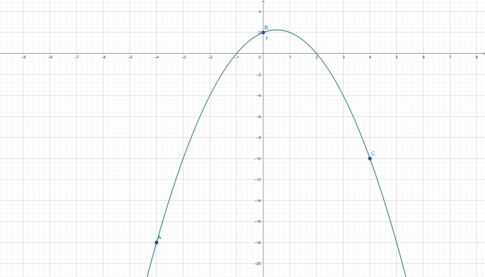
Determine a polynomial $p(x) = a_0 + a_1x + a_2x^2$ whose graph passes through the points $(-4,-18)$, $(0,2)$, and $(4,-10)$.
A polynomial with three unknown coefficients $a_0$, $a_1$, and $a_2$ passes through points $(-4,-18)$, $(0,2)$, and $(4,-10)$. Hence we have three equations
$$ \begin{align*} a_0 - 4a_1 + 16a_2 &= -18 \\ a_0\qquad\qquad\qquad &= 2 \\ a_0 + 4a_1 + 16a_2 &= -10 \end{align*} $$
Solve this linear system to determine the coefficients of the quadratic polynomial that passes through all three points.
Check Your Work
$p(x) = -x^2 + x + 2$.
Follow Along
These equations can be written in any order so we write them,
$$ \begin{align*} a_0\qquad\qquad\qquad &= 2 \\ a_0 + 4a_1 + 16a_2 &= -10 \\ a_0 - 4a_1 + 16a_2 &= -18 \end{align*} $$
Subtracting the first equation from the other two yields
$$ \begin{align*} a_0\qquad\qquad\qquad &= 2 \\ \qquad 4a_1 + 16a_2 &= -12 \\ \qquad -4a_1 + 16a_2 &= -20 \end{align*} $$
Adding the second equation to the third gives us
$$ \begin{align*} a_0\qquad\qquad\qquad &= 2 \\ \qquad 4a_1 + 16a_2 &= -12 \\ \qquad\qquad 32a_2 &= -32 \end{align*} $$
Dividing the second equation on both sides by 4, and dividing the third equation on both sides by 32 results in
$$ \begin{align*} a_0\qquad\qquad\quad &= 2 \\ \qquad a_1 + 4a_2 &= -3 \\ \qquad\qquad a_2 &= -1 \end{align*} $$
Finally, the solution follows from subtracting 4 times the third equation from the second.
$$ \begin{align*} a_0\qquad\qquad &= 2 \\ \qquad a_1 \qquad &= 1 \\ \qquad\qquad a_2 &= -1 \end{align*} $$
We now have that the unique quadratic polynomial that passes through these three points is given by
$$ y = -x^2 + x + 2 $$
1.1.5 Rectangular Linear Systems
The Shape of Linear Systems
Linear systems for which there are an equal number of equations and unknowns are called square systems. There is no law that says the number of equations and the number of unknowns has to be the same. Linear systems that have either more equations than unknowns, or more unknowns than equations are referred to as rectangular linear systems.
The system
$$ \begin{array}{rcl} 3x + 2y & = & 1 \\ x - y & = & 2 \\ 2x + 3y & = & -1 \end{array} $$
has 3 equations with 2 unknowns, the system
$$ \begin{array}{rcl} 3x + 2y - z & = & 4 \\ x + y + z & = & 3 \end{array} $$
has 2 equations and 3 unknowns, and the system
$$ \begin{array}{rcl} a_{11}x_1 + a_{12}x_2 +\ \cdots\ + a_{1n}x_n & = & b_1 \\ a_{21}x_1 + a_{22}x_2 +\ \cdots\ + a_{2n}x_n & = & b_2 \\ \\ \vdots\ \ \ \ +\ \ \ \vdots\ \ \ \ +\ \cdots\ +\ \ \ \vdots\ \ \ \ & = & \vdots \\ \\ a_{m1}x_1 + a_{m2}x_2 +\ \cdots + a_{mn}x_n & = & b_m \end{array} $$
has $m$ equations and $n$ unknowns. We will call a system of $m$ linear equations and $n$ unknowns an
Definition
System of Linear Equations
An $m\times n$ System of Linear Equations consists of a list of $m$ equations containing a total of $n$ unknowns.
Overdetermined Linear System
We will find that if there are more equations than unknowns then it is harder for the system to have any solution at all; there are just too many equations limiting the number of possible solutions until there are none. We call a system of equations with more equations than unknowns overdetermined.
Underdetermined Linear System
If there are fewer equations than unknowns, then we do not have enough information about our system to have only one solution and there will usually be infinitely many solutions. We call a system of equations with fewer equations than unknowns underdetermined.
Square Linear System
Linear systems with the same number of equations and unknowns are called square. Just like in geometry, technically all square linear systems are rectangular, but not all rectangular linear systems are square. In practice, only overdetermined or underdetermined linear systems are referred to as rectangular.
Exercise 4 - Networks
In many applications one encounters flow objects through a network or medium that restricts the flow along predetermined paths. This may be the flow of information in a stream, the flow of automobiles in traffic, the flow of current in an electrical circuit, or the flow of network data across a network. Mathematically we model these applications with a directed graph. A directed graph consists of nodes that connect edges. If the edges allow flow in either direction, then the graph is undirected. If the edges of the graph have arrows indicating direction from one node to another only, then we call the graph a directed graph.
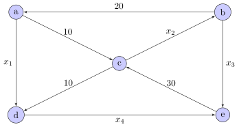
One rule of such a directed graph is that the flow into each node must equal the flow out of each node. Represent the network flow using a linear system of equations.
Check Your Work
$$ \begin{align*} x_1\qquad\qquad\qquad\ &= 10 \\ x_2 - x_3\qquad &= 20 \\ x_2\qquad\qquad &= 30 \\ x_1\qquad\qquad - x_4 &= -10 \\ x_3 + x_4 &= 30 \end{align*} $$
Follow Along
If we proceed from node $a$ to node $e$, then we can see that $x_1 + 10$ units of our object flows __out__ of node $a$ and $20$ units flows __into__ node $a$. Hence
$$ x_1 + 10 = 20 $$
Likewise at node $b$, $x_2$ units flow into node $b$ and $x_3+20$ units flows __out__ of node $b$. Continuing in this way we obtain four more equations
$$ \begin{align*} \text{node }b\ &\ &x_2 &= x_3 + 20 \\ \text{node }c\ &\ &x_2 + 10 &= 10 + 30 \\ \text{node }d\ &\ &x_1 + 10 &= x_4 \\ \text{node }e\ &\ &x_3 + x_4 &= 30 \end{align*} $$
This yields the linear system of equations
$$ \begin{align*} x_1\qquad\qquad\qquad\ &= 10 \\ x_2 - x_3\qquad &= 20 \\ x_2\qquad\qquad &= 30 \\ x_1\qquad\qquad - x_4 &= -10 \\ x_3 + x_4 &= 30 \end{align*} $$
One may write this linear system more explicitly
$$ \begin{align*} x_1 + 0x_2 + 0x_3 + 0x_4 &= 10 \\ 0x_1 +\,\ x_2 -\,\ x_3 + 0x_4 &= 20 \\ 0x_1 +\,\ x_2 + 0x_3 + 0x_4 &= 30 \\ x_1 + 0x_2 + 0x_3 -\,\ x_4 &= -10 \\ 0x_1 + 0x_2 +\,\ x_3 +\,\ x_4 &= 30 \end{align*} $$
Notice that the linear system in this exercise consists of five equations with four unknowns. This results in a $5\times 4$ linear system of equations. To draw this linear system one would need to display five (5) three-dimensional (3d) hyperplanes in four dimensional (4d) space, all intersecting at a single point.
Exercise 5 - Best-Fit Line
Consider the three data points
$$(1,2),\ (2,2),\ (3,5).$$
We want to fit a line $y=mx+b$ to these points. Each data point gives one equation: substituting $x$ and $y$ from the point yields a linear equation in the unknowns $m$ and $b$.
(a) Write down the linear system in $m$ and $b$.
(b) What is the size of this linear system? Is it square, overdetermined, or underdetermined?
(c) Try to solve the system. Use the first two equations to find $m$ and $b$, then check whether the resulting line passes through the third point. What do you conclude?
Check Your Work
(a) $m + b = 2$, $2m + b = 2$, $3m + b = 5$. (b) A $3\times 2$ overdetermined system. (c) The first two equations give $y = 2$, which misses $(3,5)$; the system is inconsistent.
Follow Along
(a) Substituting each point into $y = mx + b$:
$$ \begin{align*} m + b &= 2 \\ 2m + b &= 2 \\ 3m + b &= 5 \end{align*} $$(b) The system is $3\times 2$, three equations and two unknowns. Since there are more equations than unknowns, the linear system is overdetermined.
(c) Use the first two equations. Subtracting equation one from equation two eliminates $b$ so
$$ m=0. $$Substituting $m=0$ into equation one yields $b=2$. So the line determined by the first two equations is $y=2$, a horizontal line.
Now check whether this line passes through the third point $(3,5)$. At $x=3$ the value of the line is still $2$, not $5$. The third equation is not satisfied.
The three points are not collinear. The slope of the line that passes through points $(1,2)$ and $(2,2)$ is $0$. The slope of the line that passes through $(2,2)$ and $(3,5)$ has slope $3$. No single line passes through all three points. Hence, the linear system has no solutions; it is inconsistent.
This is the typical situation for overdetermined systems. Later in the course we will study least squares, a technique that finds the line that comes closest to all three points even though no exact line exists.
1.1.6 The Row Picture for Linear Equations
Familiar Examples
Fortunately for us there exists a straightforward geometric interpretation of a system of 2 equations and 2 unknowns. We can demonstrate the three (yes only three) types of $2\times 2$ systems and draw their graphs to illustrate what can happen.
$$ \begin{align*} 1.\quad x_1 + x_2 &= 3 &\qquad 2.\quad\ \,x_1 +\ \,x_2 &= 3 &\qquad 3.\quad x_1-x_2 &= 1 \\ x_1 - x_2 &= -1 &\qquad 3x_1 + 3x_2 &= 9 &\qquad x_1-x_2 &= -3 \end{align*} $$
This geometric interpretation is called the row picture and it was introduced to us in pre-calculus algebra class. We will expand on these definitions in section 1.1.9. Each equation in these linear systems is the equation of a line.
Definition
1. Consistent and Independent
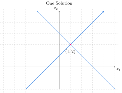
If the two lines have different slopes, they must intersect at a single point. This is a point on the plane $(x_1,\ x_2)$ that lies on both lines. This gives us a single point that makes both linear equations true. Since it is a solution to the equations of both lines, it is called a solution to the linear system.
A linear system with any solution at all, no matter how many, is called consistent.
When the two lines have different slopes, then the system is called independent.
| Linear System | Graph |
|---|---|
| $$ \begin{align*} 1.\quad x_1 + x_2 &= 3 \\ x_1 - x_2 &= -1 \end{align*} $$ |
 |
Definition
2. Consistent and Dependent
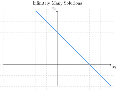
If the two lines have the same slope and the same $y$-intercept, the two lines are in fact the same line and every solution for one of the equations is also a solution for both equations. The system has infinitely many solutions.
A linear system with infinitely many solutions is still consistent.
When the two lines have the same slope, the system is called dependent.
| Linear System | Graph |
|---|---|
| $$ \begin{align*} 2.\quad\ \,x_1 + \ \,x_2 &= 3 \\ 3x_1 + 3x_2 &= 9 \end{align*} $$ |
 |
Definition
3. Inconsistent and Dependent
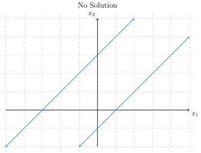
If the two lines have the same slope, but different $y$-intercepts, the two lines are parallel and never intersect. While there are infinitely many solutions to each equation; there is no point that is the solution to both equations. The system has no solutions.
A linear system with no solutions at all is called inconsistent.
When the two lines have the same slope, the system is called dependent.
| Linear System | Graph |
|---|---|
| $$ \begin{align*} 3.\quad x_1 - x_2 &= 1 \\ x_1 - x_2 &= -3 \end{align*} $$ |
 |
1.1.7 The Row Picture for Larger Linear Systems
Limitations of the Row Picture
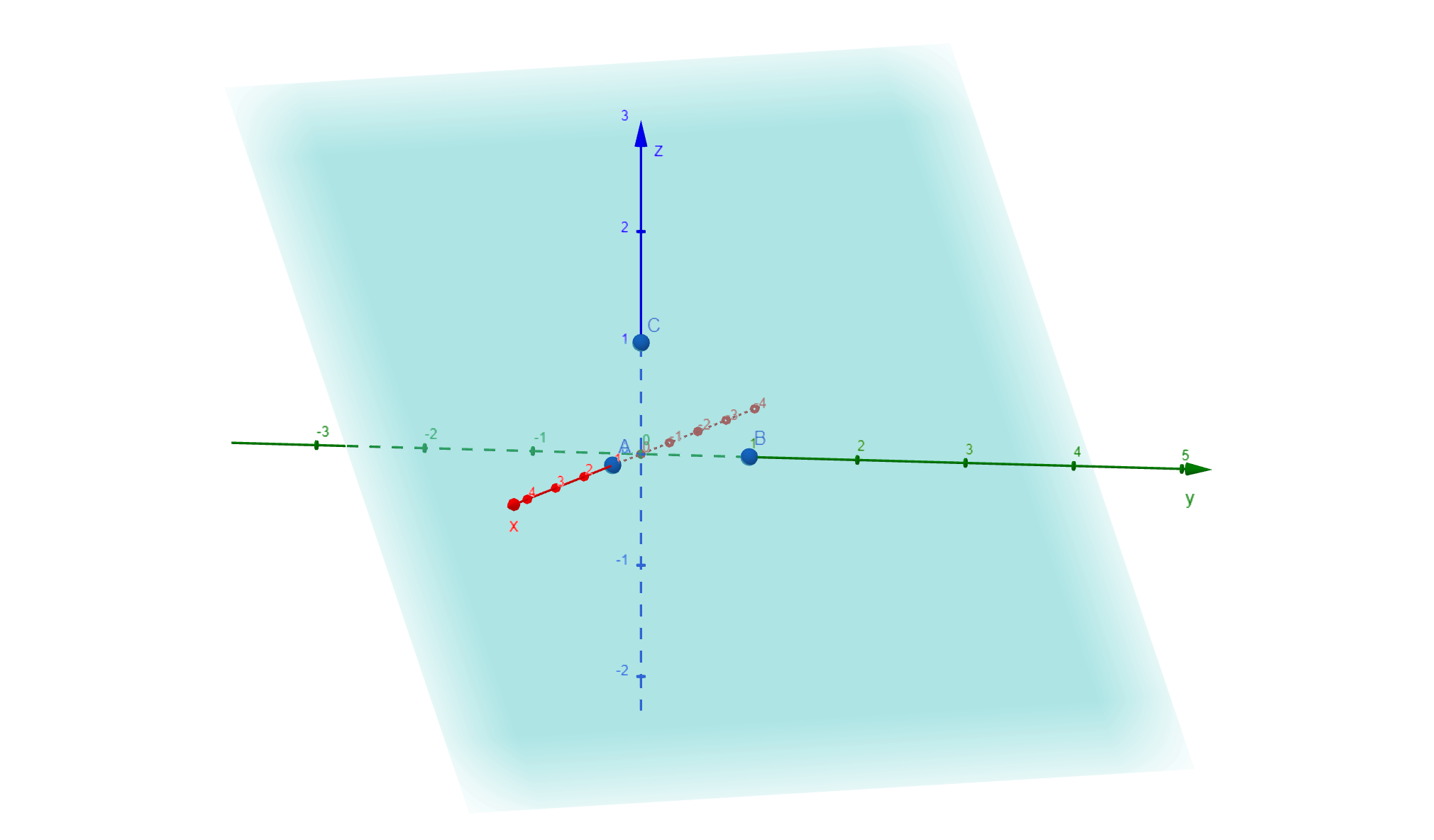
We learned in calculus that the graph of a linear equation with three unknowns can be considered a plane in three dimensional space. One may graph the plane by first plotting three points on the plane first, and then drawing the unique plane that passes through those three non co-linear points. Open the graph of the plane by clicking on the link below the graph.
| Linear System | Graph |
|---|---|
| $$ x+y+z = 1 $$ |
 |
Consider a linear system of three equations and three unknowns.
| Linear System | Graph |
|---|---|
| $$ \begin{align*} \qquad\qquad x +\,\ \ y +\,\ \ z &=\ \ 7 \\ \qquad\qquad x +\, 4y + 4z &=\ \ 25 \\ \qquad\qquad x - 4y +\,\ \ z &= -3 \end{align*} $$ |
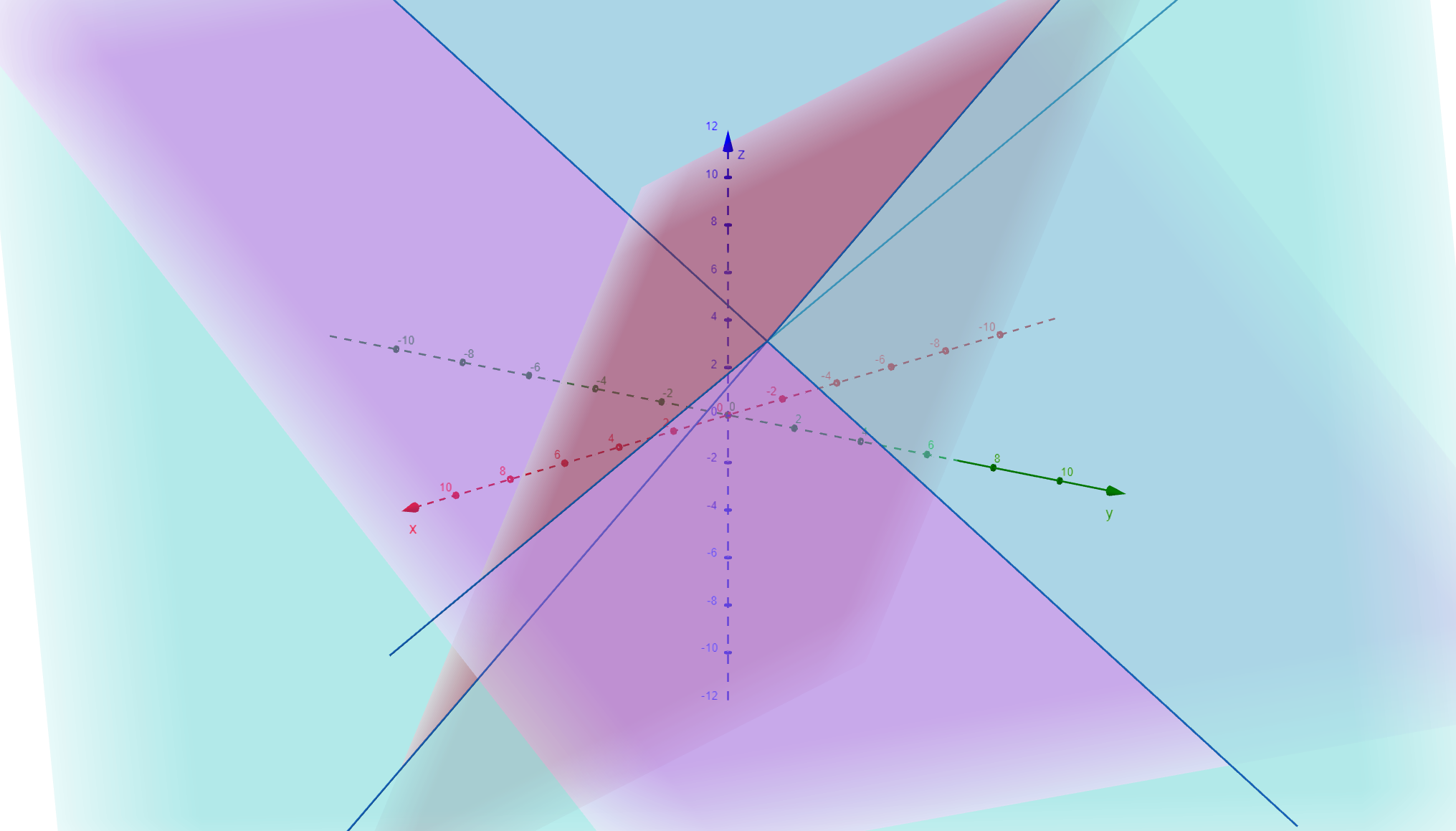 |
We run into two very impossible problems with the row picture. The use of hyperplanes and the use of substitution fails for even moderate systems with eight equations and eight unknowns. There is no chance to solve larger systems using substitution. We need the column picture and linear combinations.
1.1.8 Vectors
Before we go on we need to understand one of the new basic elements of linear algebra. We need to study a video and understand
What are Vectors Anyway?
Video Lecture 4: Vectors, what even are they?
When both scalar variables and constants appear in equations with vectors and matrices, one requires notation that distinguishes them from each other in the writing. Scalars are real or complex numbers that we already understand from our previous mathematics courses. Vectors are elements of a Vector Space. We will learn that there are many types of vector spaces. All have uses in mathematical models.
In order to denote a vector-valued variable, one needs to decorate the letter or name to distinguish it from a scalar variable or matrix.
| Decoration | Representation |
|---|---|
| Arrow over | $\overrightarrow{v_1},\ \ \overrightarrow{v_2}$ |
| Overline | $\overline{v_1},\ \ \overline{v_2}$ |
| Underline | $\underline{x},\ \ \underline{y_2}$ |
| Bold face | $\mathbf{v}_1,\ \ \mathbf{v}_2$ |
| Hat | $\ihat,\ \ \hat{\mathbf{x}}$ |
| Tilde | $\tilde{v}_1,\ \ \tilde{x}$ |
Bold face will be preferred in these online notes. Arrows, overline or underline should be used for handwritten work. A vector decorated with the "hat" or "tilde" are typically reserved for special cases, such as the canonical basis vectors $\ihat$, $\jhat$, and $\khat$ or a "changed" or shifted vector $\mathbf{x}\mapsto\tilde{\mathbf{x}}$. These will be discussed in more detail when they come up.
You must use one of the notations above to distinguish scalars from vectors in your handwritten computations. You need to learn to communicate clearly and accurately in a STEM field. All too often the future engineer that needs to accurately read your notes is you.
1.1.9 The Column Picture
A More Useful Understanding of Linear Systems
The problem with the row picture of a $2\times 2$ systems of linear equations is that it does not extend very well to larger $m\times n$ systems of linear equations. To extend our ideas of consistent and independent to larger $m\times n$ systems of linear equations, we need to view the same three systems using the column picture. Recall our three $2\times 2$ systems of linear equations
$$ \begin{align*} 1.\quad x_1 + x_2 &= 3 &\qquad 2.\quad\ \,x_1 +\ \,x_2 &= 3 &\qquad 3.\quad x_1-x_2 &= 1 \\ x_1 - x_2 &= -1 &\qquad 3x_1 + 3x_2 &= 9 &\qquad x_1-x_2 &= -3 \end{align*} $$
Let us re-write the first linear system in vector form.
$$ 1.\ \ \begin{bmatrix} x_1 + x_2 \\ x_1 - x_2 \end{bmatrix} = \begin{bmatrix} x_1 \\ x_1 \end{bmatrix} + \begin{bmatrix}\ \ x_2 \\ -x_2 \end{bmatrix} = x_1\begin{bmatrix} 1 \\ 1 \end{bmatrix} + x_2\begin{bmatrix} \ \ 1 \\ -1 \end{bmatrix} = \begin{bmatrix}\ \ 3 \\ -1 \end{bmatrix} $$
Notice that we start out with a column vector on the left side of the equation
$$ \begin{bmatrix} x_1 + x_2 \\ x_1 - x_2 \end{bmatrix} $$
This vector equals the vector on the right side of the equation
$$ \begin{bmatrix}\ \ 3 \\ -1 \end{bmatrix} $$
However, we use vector arithmetic, vector addition and scalar multiplication, to write the algebraic expression on the left-hand side of the equation as a linear combination.
$$ x_1\begin{bmatrix} 1 \\ 1 \end{bmatrix} + x_2\begin{bmatrix} \ \ 1 \\ -1 \end{bmatrix} $$
Definition
Whenever an algebraic expression multiplies vectors by scalars, and adds them together, the result is called a linear combination of vectors.
This is one of the fundamental ideas of this course. You should take the time to recognize a linear combination each time it appears in our notes, the videos, the lectures or the textbook.
Consistent and Independent
This gives us the vector equation
$$ x_1\begin{bmatrix} 1 \\ 1 \end{bmatrix} + x_2\begin{bmatrix} \ \ 1 \\ -1 \end{bmatrix} = \begin{bmatrix}\ \ 3 \\ -1 \end{bmatrix} $$
If we name our vectors $\mathbf{v}_1$ and $\mathbf{v}_2$, then we have
$$ \mathbf{v}_1 = \begin{bmatrix} 1 \\ 1 \end{bmatrix},\qquad \mathbf{v}_2 = \begin{bmatrix}\ \ 1 \\ -1 \end{bmatrix} $$
We typically name the vector on the right-hand side of the equation $\mathbf{b}$. Our system of equations can now be written
| Linear System | Graph |
|---|---|
| $$ \qquad\qquad x_1\mathbf{v}_1 + x_2\mathbf{v}_2 = \mathbf{b} $$ |
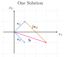 |
Since $1\,\mathbf{v}_1 + 2\,\mathbf{v}_2 = \mathbf{b}$, we have $x_1=1$ and $x_2=2$, so our unique solution is the vector
$$ \begin{bmatrix} x_1 \\ x_2 \end{bmatrix} = \begin{bmatrix} 1 \\ 2 \end{bmatrix} $$
Definition
Consistent and Linearly Independent
- When there is any linear combination of the vectors in a linear system that is equal to vector $\mathbf{b}$, the linear system is called consistent.
- When none of the vectors in a linear system is a linear combination of the other vectors, the linear system is called linearly independent.
- There will be exactly one solution to a consistent, linearly independent linear system. This solution is called unique.
Consistent and Dependent
Let us write the second linear system in vector form.
$$ \begin{bmatrix} x_1 + x_2 \\ 3x_1 + 3x_2 \end{bmatrix} = x_1\begin{bmatrix} 1 \\ 3 \end{bmatrix} + x_2\begin{bmatrix} 1 \\ 3 \end{bmatrix} = \begin{bmatrix} 3 \\ 9 \end{bmatrix} = 3\begin{bmatrix} 1 \\ 3 \end{bmatrix} $$
Notice that $\mathbf{v}_1 = \mathbf{v}_2 = \begin{bmatrix} 1 \\ 3 \end{bmatrix}$, so they are certainly linearly dependent. Notice also that $\mathbf{b} = 3\begin{bmatrix} 1 \\ 3 \end{bmatrix}$. Our vector equation becomes
$$ \left(x_1 + x_2\right)\begin{bmatrix} 1 \\ 3 \end{bmatrix} = 3\begin{bmatrix} 1 \\ 3 \end{bmatrix} $$
Thus we have
| Linear System | Graph |
|---|---|
| $$ x_1 + x_2 = 3 $$ |
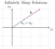 |
We obtain an equation for $x_1$ and $x_2$ that has infinitely many solutions, $x_1 + x_2 = 3$. We could plot this equation on a Cartesian plane, and the set of solutions is a line with slope $-1$ and $y$-intercept $3$. All of the points $(x_1, x_2)$ on this line gives us a solution to the linear system. This linear system has infinitely many solutions.
Definition
Consistent and Linearly Dependent
When there is any linear combination of the vectors in a linear system that is equal to vector $\mathbf{b}$, the linear system is called consistent.
If any vector in the linear system belongs to the span of the other vectors, the linear system is called linearly dependent.
There will be infinitely many solutions to a consistent, linearly dependent linear system.
Inconsistent and Dependent
Let us write the last system of linear equations in vector form.
$$ \begin{bmatrix} x_1-x_2 \\ x_1-x_2 \end{bmatrix} = \begin{bmatrix} x_1 \\ x_1 \end{bmatrix} + \begin{bmatrix} -x_2 \\ -x_2 \end{bmatrix} = x_1\begin{bmatrix} 1 \\ 1 \end{bmatrix} + x_2\begin{bmatrix} -1 \\ -1 \end{bmatrix} = \begin{bmatrix} \ \ 1 \\ -3 \end{bmatrix} $$
In this case, $\mathbf{v}_1 = \begin{bmatrix} 1 \\ 1 \end{bmatrix}$ and $\mathbf{v}_2 = \begin{bmatrix} -1 \\ -1 \end{bmatrix} = -\mathbf{v}_1$. In the language of our linear algebra videos, $\mathbf{v}_1$ and $\mathbf{v}_2$ lie on the same span. They point opposite directions but they lie on the same line so that any linear combination of vectors $\mathbf{v}_1$ and $\mathbf{v}_2$ will be on that line with slope $1$ and $y$-intercept $0$.
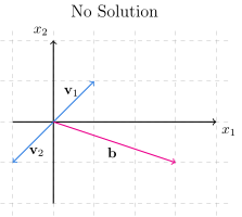
These vectors are linearly dependent because they are collinear. Since $\mathbf{b}$ is not a vector in their span, there is no linear combination of vectors $\mathbf{v}_1$ and $\mathbf{v}_2$ that will equal $\mathbf{b}$. This system of linear equations has no solution.
Definition
Inconsistent and Linearly Dependent
When there is no linear combination of our vectors $\mathbf{v}_1$ and $\mathbf{v}_2$ that equals $\mathbf{b}$, the linear system is called inconsistent.
If any vector in the linear system belongs to the span of the other vectors, the linear system is called linearly dependent.
Any inconsistent linear system will have no solutions.
The column picture is more useful because we can apply the same ideas to larger systems of $m$ equations and $n$ unknowns. Keep in mind that every linear system can have only three types of solutions. This remains true regardless of the number of equations and the number of unknowns.
Three Possible Outcomes for a Linear System
There are only three possible outcomes for the number of solutions to a system of linear equations:
- A linear system that is consistent and independent has exactly one solution.
- A linear system that is inconsistent and dependent has no solutions.
- A linear system that is consistent and dependent has infinitely many solutions.
Example 3 - Circuits

A two-loop resistor circuit with one battery and three resistors. Kirchhoff's current law states that the algebraic sum of currents at any node must be equal to zero. Hence
$$ I_1 - I_2 - I_3 = 0 $$
Kirchhoff's voltage law states that the sum of voltage drops equals the EMF supplied by sources in any loop.
$$ \begin{align*} 6I_1 + 2I_3 &= 22 \\ 4I_2 - 2I_3 &= 0 \end{align*} $$
These linear equations combine into the linear system
$$ \begin{align*} I_1 - I_2 -\ \ I_3 &= 0 \\ 6I_1\ \ \ \ \ \ \ \ + 2I_3 &= 22 \\ 4I_2 - 2I_3 &= 0 \\ \end{align*} $$
Subtracting 6 times equation one from equation two yields
$$ \begin{align*} I_1 - I_2 -\ \ I_3 &= 0 \\ 6I_2 + 8I_3 &= 22 \\ 4I_2 - 2I_3 &= 0 \end{align*} $$
Dividing both sides of equations two and three by two results in
$$ \begin{align*} I_1 - I_2 -\ \ I_3 &= 0 \\ 3I_2 + 4I_3 &= 11 \\ 2I_2 -\ \ I_3 &= 0 \end{align*} $$
Subtracting equation three from equation two produces
$$ \begin{align*} I_1 - I_2 -\ \ I_3 &= 0 \\ I_2 + 5I_3 &= 11 \\ 2I_2 -\ \ I_3 &= 0 \end{align*} $$
Subtracting two times equation two from equation three produces
$$ \begin{align*} I_1 - I_2 -\ \ I_3 &= 0 \\ I_2 + 5I_3 &= 11 \\ -11I_3 &= -22 \end{align*} $$
Therefore
$$ \begin{align*} I_3 &= 2 \\ I_2 &= 11 - 5(2) = 1 \\ I_1 &= 2 + 1 = 3 \end{align*} $$
Thus $I_1 = 3\,\textrm{A}$, $I_2=1\,\textrm{A}$, and $I_3=2\,\textrm{A}$.
Exercise 6 - Recognizing Dependence
Consider the vectors
$$\mathbf{v}_1 = \begin{bmatrix} 2 \\ 1 \end{bmatrix},\quad\mathbf{v}_2 = \begin{bmatrix} -4 \\ -2 \end{bmatrix}$$
(a) Without computing any elimination, decide whether there exist scalars $x_1$, $x_2$ such that
$$x_1\mathbf{v}_1 + x_2\mathbf{v}_2 = \mathbf{b},\quad\mathbf{b}=\begin{bmatrix} 3 \\ 1 \end{bmatrix}.$$If such scalars exist, are they unique? If they do not exist, explain geometrically why not.
(b) Repeat part (a) with the same $\mathbf{v}_1$, $\mathbf{v}_2$ but a different right-hand side:
$$\mathbf{b} = \begin{bmatrix} 6 \\ 3 \end{bmatrix}$$Check Your Work
(a) No such scalars. The system is inconsistent and dependent. (b) Infinitely many such scalars. The system is consistent and dependent.
Follow Along
Observe vectors $\mathbf{v}_1$ and $\mathbf{v}_2$. Notice that $\mathbf{v}_2 = -2\mathbf{v}_1$, so vectors $\mathbf{v}_1$ and $\mathbf{v}_2$ are collinear, and lie on the same line through the origin with slope $\frac{1}{2}$. The span is just that line, not the whole plane:
$$\textrm{Span}\left\{\mathbf{v}_1,\mathbf{v}_2\right\} = \left\{ t\begin{bmatrix} 2 \\ 1 \end{bmatrix}\,:\,t\in\mathbb{R} \right\}$$
By the definitions of this section $\mathbf{v}_1$ and $\mathbf{v}_2$ are linearly dependent.
(a) Is $\mathbf{b} = \begin{bmatrix} 3 \\ 1 \end{bmatrix}$ on the line $y = \frac{x}{2}$? At $x=3$ the value of $y$ on the line is $\frac{3}{2}$, not $1$. So $\mathbf{b}$ is not in the span of $\mathbf{v}_1$ and $\mathbf{v}_2$, and no linear combination of them will produce $\mathbf{b}$. This linear system is inconsistent and dependent; it has no solutions.
(b) Is $\mathbf{b} = \begin{bmatrix} 6 \\ 3 \end{bmatrix}$ on the line $y = \frac{x}{2}$? At $x=6$ the value of $y$ on the line is $3$. Yes, vector $\mathbf{b}$ lies in the span. The system is consistent and dependent; it has infinitely many solutions.
To see the solutions explicitly, the vector equation $x_1\mathbf{v}_1 + x_2\mathbf{v}_2 = \mathbf{b}$ becomes
$$x_1\begin{bmatrix} 2 \\ 1 \end{bmatrix} + x_2\begin{bmatrix} -4 \\ -2 \end{bmatrix} = \begin{bmatrix} 6 \\ 3 \end{bmatrix},$$which reduces to the single equation $x_1 - 2x_2 = 3$ (the two component equations are multiples of each other). Any pair $(x_1,x_2)$ on the line solves the system. For instance $(x_1,x_2) = (3,0)$, $(5,1)$, and $(1,-1)$ all work.
1.1.10 Linear Combination and Span
Span
Start with this video to gain a geometrical understanding of linear combinations and the span of a set of vectors.
Video Lecture 5: SpanDefinition
Span
The span of a set of vectors $S = \left\{ \mathbf{v}_1,\ \mathbf{v}_2,\ \dots,\ \mathbf{v}_k \right\}$ is the set of all possible linear combinations of the vectors in the set $S$.
1. The Span of One Vector
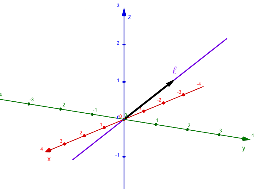
Geometrically the span of one vector is a line.
2. The Span of Two Dependent Vectors
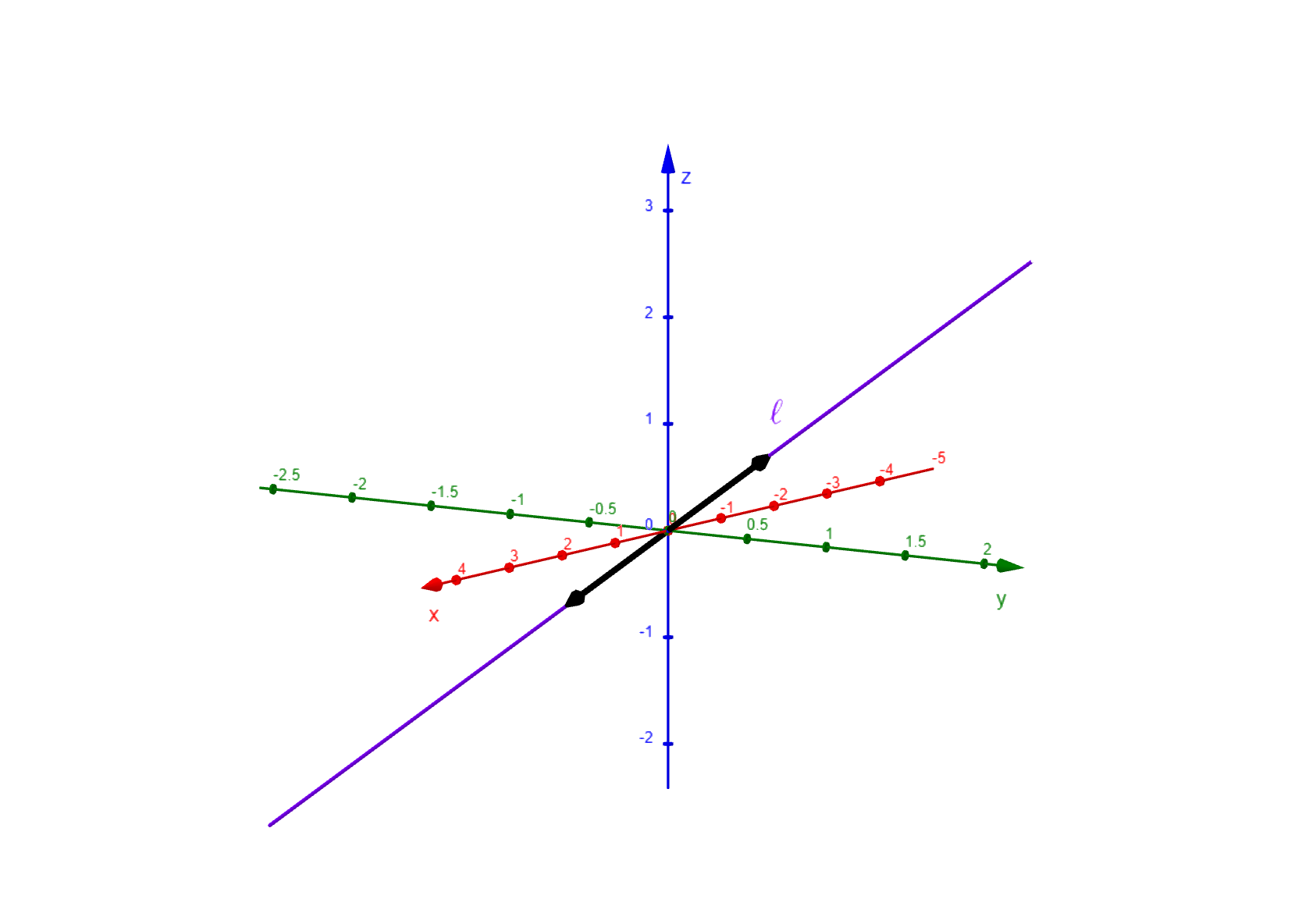
The span of two vectors is more complicated. If two vectors are collinear, they belong to the same span and they are constant multiples of each other.
If two vectors point in different directions, then their span, the set of all possible linear combinations of the two vectors, is a plane.
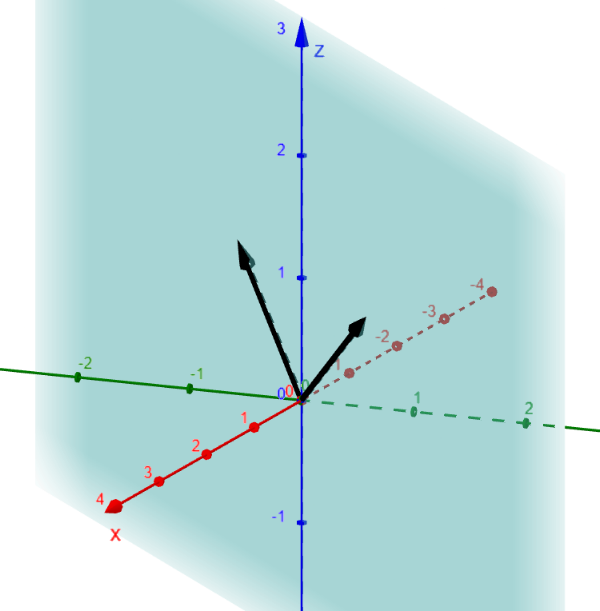
- The span of two linearly independent vectors is a plane.
- The span of two linearly dependent or collinear vectors is still just a line.
3. The Span of Three Vectors
The span of three vectors gets even more complicated because we have several possible outcomes.
(a) The Span of 3 Dependent Vectors
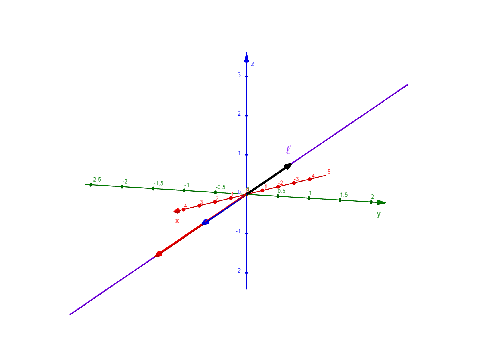
Three linearly dependent vectors are all scalar multiples of each other. They all point in the same or opposite directions. Hence every linear combination of them points along the same line.
(b) The Span of Two Independent Vectors and One Dependent Vector
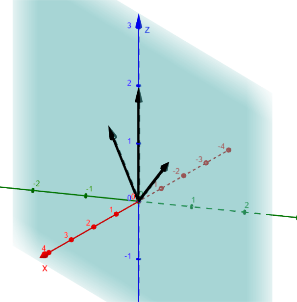
When only two of the three vectors point in a new direction, the third vector is a linear combination of the other two. This results in a plane because the third vector is just another vector on the plane spanned by linearly independent vectors.
(c) The Span of 3 Independent Vectors
The span of three linearly independent vectors is all of three-dimensional space. Each independent direction that a vector points adds to the dimension of their span.
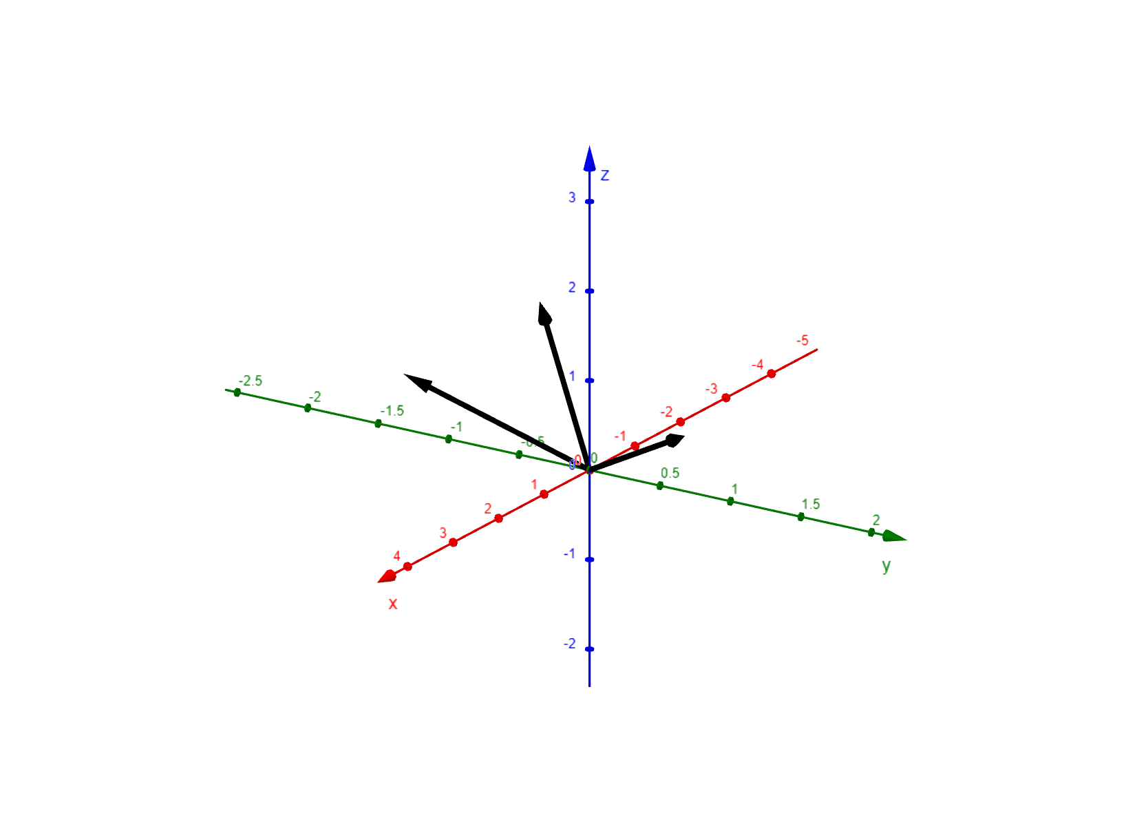
- The span of three linearly independent vectors is three dimensional space because linearly independent vectors all point in different directions.
- The span of three collinear vectors is still a line.
- The span of two linearly independent vectors and one dependent vector is a plane.
We will need to build more experience with vectors in order to study the geometrical relationships between larger numbers of vectors in very large dimensional problems.
Exercise 7 - Spanning Questions in $\mathbb{R}^3$
Consider the vectors in $\mathbb{R}^3$
$$\mathbf{v}_1 = \begin{bmatrix} 1 \\ 2 \\ 0 \end{bmatrix},\ \mathbf{v}_2 = \begin{bmatrix} 0 \\ 1 \\ 1 \end{bmatrix}.$$
(a) Do $\mathbf{v}_1$ and $\mathbf{v}_2$ span all of $\mathbb{R}^3$? Why or why not?
(b) Describe the span of $\left\{\mathbf{v}_1,\mathbf{v}_2\right\}$ geometrically. What kind of object is it?
(c) Is $\mathbf{b}=\begin{bmatrix} 1 \\ 3 \\ 1 \end{bmatrix}$ in the span of $\left\{\mathbf{v}_1,\mathbf{v}_2\right\}$? If so, find scalars $x_1$, $x_2$ such that $x_1\mathbf{v}_1 + x_2\mathbf{v}_2 = \mathbf{b}$.
(d) Is $\mathbf{c} = \begin{bmatrix} 1 \\ 1 \\ 1 \end{bmatrix}$ in the span of $\left\{\mathbf{v}_1,\mathbf{v}_2\right\}$? Justify your answer.
Check Your Work
(a) No. (b) A plane through the origin in $\mathbb{R}^3$. (c) Yes, with $x_1 = 1$ and $x_2 = 1$. (d) No.
Follow Along
(a) Two vectors can span at most a two-dimensional subspace of $\mathbb{R}^3$. To span all of $\mathbb{R}^3$ we would need at least three linearly independent vectors. Since we have only two, $\textrm{Span}\left\{\mathbf{v}_1,\mathbf{v}_2\right\}$ is at most a plane that passes through the origin.
(b) The vectors $\mathbf{v}_1$ and $\mathbf{v}_2$ are not scalar multiples of one another, so they are linearly independent. Their span is therefore exactly a plane through the origin in $\mathbb{R}^3$; the plane containing $\mathbf{v}_1$ and $\mathbf{v}_2$.
(c) Asking whether $\mathbf{b}$ is in the span means asking whether the vector equation $x_1\mathbf{v}_1 + x_2\mathbf{v}_2 = \mathbf{b}$ has a solution.
The vector equation $$ x_1\begin{bmatrix} 1 \\ 2 \\ 0 \end{bmatrix} + x_2\begin{bmatrix} 0 \\ 1 \\ 1 \end{bmatrix} = \begin{bmatrix} 1 \\ 3 \\ 1 \end{bmatrix}$$results in the linear system
$$\begin{align*} x_1\ \ \ \ \ \ \ \ \ &= 1 \\ 2x_1 + x_2 &= 3 \\ x_2 &= 1 \end{align*}$$From the first equation, $x_1 = 1$, and from the third, $x_2 = 1$. Checking the second equation: $2(1) + 1(1) = 3\ \checkmark$.
The system is consistent, so $\mathbf{b}$ is in the span of $\{\mathbf{v}_1, \mathbf{v}_2\}$, with $x_1 = 1$ and $x_2 = 1$. That is,
$$\mathbf{b} = \mathbf{v}_1 + \mathbf{v}_2.$$(d) Set up the same vector equation with $\mathbf{c}$ in place of $\mathbf{b}$:
$$\begin{align*} x_1\ \ \ \ \ \ \ \ \ &= 1 \\ 2x_1 + x_2 &= 1 \\ x_2 &= 1 \end{align*}$$The first equation forces $x_1 = 1$; the third forces $x_2 = 1$. Checking the second equation: $2(1) + 1(1) = 3$, but the equation requires it to equal $1$; a contradiction. The system is inconsistent. There are no scalars satisfying $x_1\mathbf{v}_1 + x_2\mathbf{v}_2 = \mathbf{c}$, so $\mathbf{c}$ is not in the span of $\{\mathbf{v}_1, \mathbf{v}_2\}$; it lies off the plane.
The span of $\{\mathbf{v}_1, \mathbf{v}_2\}$ is a plane through the origin in $\mathbb{R}^3$. Some vectors in $\mathbb{R}^3$ (like $\mathbf{b}$) lie on this plane and can be written as a linear combination of $\mathbf{v}_1$ and $\mathbf{v}_2$; others (like $\mathbf{c}$) do not. Whether the system $x_1 \mathbf{v}_1 + x_2 \mathbf{v}_2 = \mathbf{d}$ has a solution depends entirely on whether $\mathbf{d}$ happens to lie on this plane.
1.1.11 Solving Systems of Linear Equations
Solving Systems of Linear Equations
In our previous algebra classes, we solved a system of two equations and two unknowns using either substitution or elimination. Using the method of substitution becomes horrible when trying to solve larger systems of linear equations. Fortunately, the method of elimination works very well for even very large systems of linear equations.
Example 4 - Elimination Method
Let us consider a system of equations and use the elimination method to solve it.
$$ \begin{align*} 2x_1 + 3x_2 + \ \ x_3 &= \ \ 4 \\ 3x_1 - \ \ x_2 - 3x_3 &= -1 \\ x_1 + 2x_2 + \ \ x_3 &= \ \ 3 \end{align*} $$
We want to determine whether there is one solution, no solutions, or infinitely many solutions. We will not know the number of solutions until we solve the linear system. We will call the collection of solutions a set of solutions. A set of solutions can have one solution in the set, no solutions in the set, or infinitely many solutions in the set.
If we are going to use elimination, the arithmetic will work out better if the coefficient of $x_1$ is a $1$ in the first equation. It does not matter what order the equations appear in the system. Let us swap the first and the last equation
$$ \begin{align*} x_1 + 2x_2 + \ \ x_3 &= \ \ 3 \\ 3x_1 - \ \ x_2 - 3x_3 &= -1 \\ 2x_1 + 3x_2 + \ \ x_3 &= \ \ 4 \end{align*} $$
If we change the order of the equations then technically we have a different system of equations, but they will have the same set of solutions. We call these two systems of linear equations equivalent when they have the same set of solutions.
Next, we must eliminate the first variable $x_1$ from the second two equations. To accomplish this task we will multiply the first equation on both sides by the nonzero number $3$. This gives us a new system of equations
$$ \begin{align*} 3x_1 + 6x_2 + 3x_3 &= \ \ 9 \\ 3x_1 - \ \ x_2 - 3x_3 &= -1 \\ 2x_1 + 3x_2 + \ \ x_3 &= \ \ 4 \end{align*} $$
The graph of the first equation is still the same plane in three-dimensional space, so the system of equations has the same set of solutions. Thus, this new system is also an equivalent system of equations. We only point this out currently to illustrate that multiplying one of the equations on both sides by the same nonzero number does not change the set of solutions of the system of equations. We really want to add $-3$ times the first equation to the second equation. This results in
$$\begin{align*} -3x_1 - 6x_2 - \ 3x_3 &= -9 \\ \ 3x_1 - \ \ x_2 - 3x_3 &= -1 \\ \end{align*} $$
Adding these two equation yields the equation
$$ -7x_2 - 6x_3 = -10. $$
Now we have the equivalent linear system of equations
$$ \begin{align*} x_1 + 2x_2 + \ \ x_3 &= \ \ 3 \\ -7x_2 - 6x_3 &= -10 \\ 2x_1 + 3x_2 + \ \ x_3 &= \ \ 4 \end{align*} $$
It may not be apparent at this time but adding a nonzero multiple of one equation to another equation results in an equivalent linear system of equations; that is the two systems of equations have the same set of solutions.
We can also add $-2$ times the first equation to the third equation to obtain
$$ \begin{align*} x_1 + 2x_2 + \ \ x_3 &= \ \ 3 \\ -7x_2 - 6x_3 &= -10 \\ -x_2 - \ \ x_3 &= -2 \end{align*} $$
At this point we want to make our arithmetic as simple as possible so we will multiply both sides of the second equation by $-1$, and multiply both sides of the third equation by $-1$ to get the equivalent linear system
$$ \begin{align*} x_1 + 2x_2 + \ \ x_3 &= 3 \\ 7x_2 + 6x_3 &= 10 \\ x_2 + \ \ x_3 &= 2 \end{align*} $$
As in the first step, it would help to swap the second equation and the third equation. This will give us the equivalent linear system
$$ \begin{align*} x_1 + 2x_2 + \ \ x_3 &= 3 \\ x_2 + \ \ x_3 &= 2 \\ 7x_2 + 6x_3 &= 10 \end{align*} $$
Now we need to eliminate the variable $x_2$ from the third equation. Adding $-7$ times the second equation to the third equation yields
$$ \begin{align*} x_1 + 2x_2 + \ \ x_3 &= 3 \\ x_2 + \ \ x_3 &= 2 \\ -x_3 &= -4 \end{align*} $$
Multiplying both sides of the third equation by $-1$ gives us the equivalent linear system
$$ \begin{align*} x_1 + 2x_2 + \ \ x_3 &= 3 \\ x_2 + \ \ x_3 &= 2 \\ x_3 &= 4 \end{align*} $$
Now we have an equivalent linear system of equations with a special structure to the equations. This is called strict triangular form. I hope you can see the triangle on the left side of the equation. It will become more obvious when we write the linear system using matrices. The advantage of strict triangular form is that we can readily solve the system of equations using backward substitution. We start at the last equation and determine that
$$ x_3 = 4. $$
Using the value of $x_3$ we can substitute the value $4$ in the second equation for $x_3$ to obtain
$$ x_2 + 4 = 2. $$
Subtracting $4$ from both sides of the second equation yields
$$ x_2 = -2. $$
Substituting the values of $x_3$ and $x_2$ into the first equation gives us
$$ x_1 + 2(-2) + 4 = 3. $$
Using this equation we determine that
$$ x_1 = 3. $$
Thus our set of solutions has only one vector in the set,
$$ \begin{bmatrix} x_1 \\ x_2 \\ x_3 \end{bmatrix} = \begin{bmatrix}\ \ 3 \\ -2 \\ \ \ 4 \end{bmatrix} = \langle\, 3,\ -2,\ 4 \,\rangle $$
Notice that we found the solution using just three basic operations, and that each basic operation results in an equivalent linear system of equations.
Elementary Row Operations
$$ \begin{array}{|l|l|} \hline \text{Type} & \text{Operation} \\ \hline \textbf{Type I} & \text{Interchange two equations} \\ \hline \textbf{Type II} & \text{Multiply an equation on both sides by a nonzero number} \\ \hline \textbf{Type III} & \text{Add a multiple of one equation to another equation} \\ \hline \end{array} $$
1.1.12 Exercises
More Exercises
Exercise 8 - Network Flow
Using the elementary row operations from Example 4, solve the system created in Exercise 4.
Check Your Work
$x_1 = 10$, $x_2 = 30$, $x_3 = 10$, and $x_4 = 20$.
Follow Along
$$ \begin{align*} x_1\qquad\qquad\qquad\ &= 10 \\ x_2 - x_3\qquad &= 20 \\ x_2\qquad\qquad &= 30 \\ x_1\qquad\qquad - x_4 &= -10 \\ x_3 + x_4 &= 30 \end{align*} $$
We can display these equations in any order.
$$ \begin{align*} x_1\qquad\qquad\qquad\ &= 10 \\ x_2\qquad\qquad\ \ &= 30 \\ x_2 - x_3\qquad\ &= 20 \\ x_1\qquad\qquad - x_4 &= -10 \\ x_3 + x_4 &= 30 \end{align*} $$
Subtracting the first equation from the fourth equation simplifies the fourth equation,
$$ \begin{align*} x_1\qquad\qquad\qquad\ &= 10 \\ x_2\qquad\qquad\ \ &= 30 \\ x_2 - x_3\qquad\ &= 20 \\ \qquad\qquad\qquad - x_4 &= -20 \\ x_3 + x_4 &= 30 \end{align*} $$
Subtracting the second equation from the third equation, and adding the fourth equation to the fifth equation results in
$$ \begin{align*} x_1\qquad\qquad\qquad\ &= 10 \\ x_2\qquad\qquad\ &= 30 \\ -x_3\qquad &= -10 \\ -x_4 &= -20 \\ x_3 \qquad &= 10 \end{align*} $$
Multiplying both sides of equations three and four on both sides by -1 and realizing that equation three and equation five are equivalent yields the solution,
$$ \begin{align*} x_1\qquad\qquad\qquad\ &= 10 \\ x_2\qquad\qquad &= 30 \\ x_3\qquad &= 10 \\ x_4 &= 20 \end{align*} $$
Exercise 9 - Cubic Polynomial Fit
Find a cubic polynomial $p(x) = a_0 + a_1x + a_2x^2 + a_3x^3$ that passes through the points $(-1,0)$, $(0,1)$, $(1,0)$, and $(2,-3)$.
Check Your Work
$p(x) = 1 - x^2$.
Follow Along
Evaluating our polynomial at each point one obtains
$$ \begin{align*} p(-1) = a_0 -\ \ a_1 +\ \ a_2 -\ \ a_3 &= 0 \\ p(0) = a_0\qquad\qquad\qquad\qquad &= 1 \\ p(1) = a_0 +\ \ a_1 +\ \ a_2 +\ \ a_3 &= 0 \\ p(2) = a_0 + 2a_1 + 4a_2 + 8a_3 &= -3 \end{align*} $$
Permuting equations one and two produces
$$ \begin{align*} a_0\qquad\qquad\qquad\qquad &= 1 \\ a_0 -\ \ a_1 +\ \ a_2 -\ \ a_3 &= 0 \\ a_0 +\ \ a_1 +\ \ a_2 +\ \ a_3 &= 0 \\ a_0 + 2a_1 + 4a_2 + 8a_3 &= -3 \end{align*} $$
Subtracting the first equation from the other three yields
$$ \begin{align*} a_0\qquad\qquad\qquad\qquad &= 1 \\ -a_1 +\ \ a_2 -\ \ a_3 &= -1 \\ a_1 +\ \ a_2 +\ \ a_3 &= -1 \\ 2a_1 + 4a_2 + 8a_3 &= -4 \end{align*} $$
Adding equation two to equation three, and two times equation two to equation four results in
$$ \begin{align*} a_0\qquad\qquad\qquad\qquad &= 1 \\ -a_1 +\,\ \ a_2 -\ \ a_3 &= -1 \\ 2a_2\,\qquad\ \ &= -2 \\ 6a_2 + 6a_3 &= -6 \end{align*} $$
Now divide both sides of equation three by two, and both sides of equation four by six to get
$$ \begin{align*} a_0\qquad\qquad\qquad\quad &= 1 \\ -a_1 +\ \ a_2 - a_3 &= -1 \\ a_2\qquad\ &= -1 \\ a_2 + a_3 &= -1 \end{align*} $$
Subtracting equation three from equations two and four generates
$$ \begin{align*} a_0\qquad\qquad\qquad\quad &= 1 \\ -a_1\qquad - a_3 &= 0 \\ a_2\qquad\ &= -1 \\ a_3 &= 0 \end{align*} $$
Adding equation three to equation two simplifies to
$$ \begin{align*} a_0\qquad\qquad\qquad\quad &= 1 \\ -a_1\qquad\qquad &= 0 \\ a_2\qquad\ &= -1 \\ a_3 &= 0 \end{align*} $$
Finally multiplying both sides of equation two by negative one gives rise to
$$ \begin{align*} a_0\qquad\qquad\qquad &= 1 \\ a_1\qquad\qquad &= 0 \\ a_2\qquad\ &= -1 \\ a_3 &= 0 \end{align*} $$
As a result, the cubic polynomial that passes through the four points is the polynomial $p(x) = 1 - x^2$. Notice that although we set up a cubic, the linear system tells us $a_3 = 0$. The four points happen to lie on a quadratic, so no genuine cubic term is needed.
Exercise 10 - Diet/Nutrition
A nutritionist is designing a meal that combines three foods: oats, milk, and almonds. Each serving provides the following per-serving nutrient amounts:
| Oats | Milk | Almonds | |
|---|---|---|---|
| Protein(g) | 5 | 8 | 6 |
| Calcium(mg) | 20 | 300 | 75 |
| Iron(mg) | 2 | 0 | 1 |
Let $x_1$, $x_2$, $x_3$ denote the number of servings of oats, milk, and almonds in the meal. The nutritionist wants the meal to provide exactly 24 g of protein and 450 mg of calcium.
(a) Write down the linear system for $x_1$, $x_2$, $x_3$.
(b) What is the size of this linear system? Is it square, overdetermined, or underdetermined?
(c) Eliminate $x_1$ between the two equations. Solve for $x_2$ in terms of $x_3$, and then for $x_1$ in terms of $x_3$. Describe the set of all solutions.
(d) A solution is physically meaningful only if every $x_i \geq 0$ (you cannot have a negative number of servings). For which values of $x_3$ does the solution from Part (c) satisfy $x_1 \geq 0$, $x_2 \geq 0$, and $x_3 \geq 0$? Give one physically meaningful example.
Check Your Work
(a) $5x_1 + 8x_2 + 6x_3 = 24$ and $20x_1 + 300x_2 + 75x_3 = 450$. (b) A $2\times 3$ underdetermined system. (c) A one-parameter family of solutions. (d) $0 \le x_3 \le 3$.
Follow Along
(a) Each row of the table gives one equation. Using protein and calcium:
$$\begin{align*} 5x_1 +\ \ \ \ 8x_2 +\ \ 6x_3 &= 24 \\ 20x_1 + 300x_2 + 75x_3 &= 450 \end{align*}$$(b) The system has $2$ equations and $3$ unknowns, a $2 \times 3$ linear system. Since there are fewer equations than unknowns, the linear system is underdetermined.
(c) Multiply the first equation by $4$ to align the $x_1$ coefficient with the second equation.
$$\begin{align*} 20x_1 +\ \ 32x_2 + 24x_3 &= 96 \\ 20x_1 + 300x_2 + 75x_3 &= 450 \end{align*}$$Subtracting the first from the second eliminates $x_1$.
$$ 268x_2 + 51x_3 = 354 $$Solve for $x_2$
$$ x_2 = \frac{354 - 51x_3}{268}. $$Treat $x_3$ as a free parameter. Once $x_3$ is chosen, $x_2$ is determined, and substituting back into the first equation gives $x_1$
$$\begin{align*} 5x_1 + 8\left(\frac{354 - 51x_3}{268}\right) + 6x_3 &= 24 \\ 5x_1 + 2\left(\frac{354 - 51x_3}{67}\right) + 6x_3 &= 24 \\ 5x_1 + \frac{708 - 102x_3}{67} + \frac{402x_3}{67} &= \frac{1608}{67} \\ \\ 5x_1 + \frac{708 + 300x_3}{67} &= \frac{1608}{67} \\ 5x_1 &= \frac{900 - 300x_3}{67} \\ x_1 &= \frac{180 - 60x_3}{67} \\ \end{align*}$$There are infinitely many solutions. The solution set is a one-parameter family:
$$\left\{ \left( \frac{180 - 60x_3}{67},\, \frac{354 - 51x_3}{268},\,x_3 \right) \,:\,x_3\in\mathbb{R} \right\}$$(d) The mathematical solution set is an entire line, but most points on that line are physically meaningless. We need $x_1$,$x_2$,$x_3\ge 0$ simultaneously.
- $x_3\ge 0$ is given as the parameter range.
- $x_2\ge 0$ requires $354 - 51x_3\ge 0$, or $x_3\le \frac{354}{51} = 6\frac{48}{51}$
- $x_1\ge 0$ requires $180 - 60x_3\ge 0$, or $x_3\le 3$
Hence $0 \le x_3 \le 3$.
One concrete example would be to take $x_3=2$ (two servings of almonds).
$$\begin{align*} x_2 = \frac{354 - 102}{268} &\approx 0.94 \\ x_1 = \frac{180 - 120}{67} &\approx 0.90 \\ \\ 5\left(\frac{60}{67}\right) + 8\left(\frac{63}{67}\right) + 6(2) &= 24 \textrm{ g}\text{ of protein} \\ 20\left(\frac{60}{67}\right) + 300\left(\frac{63}{67}\right) + 75(2) &= 450 \textrm{ mg}\text{ of calcium} \end{align*}$$The meal "about $0.9$ servings of oats + $0.94$ servings of milk + $2$ servings of almonds" delivers $24$ g protein and $450$ mg calcium.
1.1.13 True/False Questions
Deciding a Claim
For each statement, decide whether it is true or false. A statement that is only sometimes true counts as false. When a statement is true, give a general argument. When it is false, give a specific counterexample and verify that it fails. Throughout, all vectors and coefficients are real.
1. If a linear system has more equations than unknowns, then it has no solution.
2. If a linear system has two different solutions, then it has infinitely many solutions.
3. The equation $x_1 x_2 + x_3 = 5$ is a linear equation in $x_1$, $x_2$, and $x_3$.
4. Any two vectors in $\mathbb{R}^2$ span $\mathbb{R}^2$.
5. If the two columns of a $2 \times 2$ linear system are linearly dependent, then the system is inconsistent.
6. Performing an elementary row operation on a linear system can change its solution set.
7. An underdetermined linear system always has infinitely many solutions.
8. If three planes in $\mathbb{R}^3$ have no point common to all three, then the corresponding linear system is inconsistent.
9. The span of two linearly independent vectors in $\mathbb{R}^3$ is a plane through the origin.
Check Your Work
1. False. 2. True. 3. False. 4. False. 5. False.
6. False. 7. False. 8. True. 9. True.
Follow Along
1. False. Consider the overdetermined system
$$ \begin{align*} x_1 &= 1 \\ 2x_1 &= 2 \end{align*} $$
Two equations, one unknown, and $x_1 = 1$ satisfies both. Overdetermined systems are usually inconsistent, and usually is not always.
2. True. Suppose $\mathbf{u}$ and $\mathbf{v}$ are distinct solutions and let $t$ be any real number. Put $\mathbf{w} = (1-t)\mathbf{u} + t\mathbf{v}$. Take any equation of the system, say $a_1 x_1 + \cdots + a_n x_n = b$. Because the left side is linear in the unknowns,
$$ \sum_{i=1}^{n} a_i w_i = (1-t)\sum_{i=1}^{n} a_i u_i + t\sum_{i=1}^{n} a_i v_i = (1-t)b + tb = b $$
So $\mathbf{w}$ satisfies every equation. Distinct values of $t$ give distinct $\mathbf{w}$ because $\mathbf{u} \neq \mathbf{v}$, and there are infinitely many choices of $t$. This is why a linear system has either no solution, exactly one, or infinitely many, and never exactly two.
3. False. The term $x_1 x_2$ is a product of two unknowns. A linear equation permits only a constant multiple of each unknown, added together.
4. False. Take $\mathbf{v}_1 = (2,1)^T$ and $\mathbf{v}_2 = (-4,-2)^T$. Since $\mathbf{v}_2 = -2\mathbf{v}_1$, every linear combination is a multiple of $\mathbf{v}_1$, so the span is the line $x_2 = x_1/2$. The vector $(3,1)^T$ does not lie on that line, so the two vectors do not span $\mathbb{R}^2$.
5. False. Use the same two columns as in statement 4. With $\mathbf{b} = (3,1)^T$ the system is inconsistent, but with $\mathbf{b} = (6,3)^T$ it reduces to the single equation $x_1 - 2x_2 = 3$ and has infinitely many solutions. Dependent columns tell you the system is not independent; they do not tell you whether it is consistent.
6. False. Each of the three elementary row operations is reversible: an interchange is undone by the same interchange, scaling by $c \neq 0$ is undone by scaling by $1/c$, and adding $c$ times one equation to another is undone by subtracting it. So any solution of the original system satisfies the new one and conversely, and the two systems have exactly the same solution set. That is the entire justification for solving a system by elimination.
7. False. Consider
$$ \begin{align*} x_1 + x_2 + x_3 &= 0 \\ x_1 + x_2 + x_3 &= 1 \end{align*} $$
Two equations, three unknowns, and no solution at all, since no triple can make the same expression equal both $0$ and $1$. Underdetermined systems have either no solution or infinitely many, never exactly one.
8. True. A solution of the system is precisely a point lying on all three planes simultaneously. If no such point exists, the system has no solution and is inconsistent by definition.
9. True. Let $\mathbf{v}_1$ and $\mathbf{v}_2$ be linearly independent. Every linear combination $c_1\mathbf{v}_1 + c_2\mathbf{v}_2$ lies in the plane determined by the two directions, and taking $c_1 = c_2 = 0$ shows the origin belongs to the span. Independence keeps the two directions distinct, so the span is genuinely two-dimensional rather than a line. Compare Figure 13.
1.1.14 Multiple Choice Questions
Check All That Apply
Each question below may have more than one correct choice. Check every box that applies. No justification is required.
1. Which of the following are linear equations in $x_1$, $x_2$, and $x_3$?
$\square\ $ $2x_1 - 3x_2 + x_3 = 7$
$\square\ $ $x_1 + \dfrac{1}{x_2} = 4$
$\square\ $ $\sqrt{5}\,x_1 - x_3 = 0$
$\square\ $ $x_1 x_3 + x_2 = 1$
$\square\ $ $\pi x_2 = e$
2. Which of the following describe the system below?
$$ \begin{align*} x_1 + 2x_2 &= 3 \\ 2x_1 + 4x_2 &= 6 \end{align*} $$
$\square\ $ Consistent
$\square\ $ Inconsistent
$\square\ $ Independent
$\square\ $ Dependent
$\square\ $ Has exactly one solution
$\square\ $ Has infinitely many solutions
3. Which of the following sets of vectors span $\mathbb{R}^2$?
$\square\ $ $\left\{ (1,0)^T,\ (0,1)^T \right\}$
$\square\ $ $\left\{ (1,2)^T,\ (2,4)^T \right\}$
$\square\ $ $\left\{ (1,1)^T,\ (1,-1)^T \right\}$
$\square\ $ $\left\{ (0,0)^T,\ (3,5)^T \right\}$
$\square\ $ $\left\{ (1,2)^T,\ (2,1)^T,\ (3,3)^T \right\}$
4. Which of the following are elementary row operations?
$\square\ $ Interchange two equations
$\square\ $ Multiply an equation by a nonzero constant
$\square\ $ Multiply an equation by zero
$\square\ $ Add a multiple of one equation to another
$\square\ $ Square both sides of an equation
Check Your Work
1. The first, third, and fifth.
2. Consistent, dependent, and has infinitely many solutions.
3. The first, third, and fifth.
4. Interchange two equations; multiply an equation by a nonzero constant; add a multiple of one equation to another.
1.1.15 Challenge Exercises
Problems Spanning the Whole Section
These exercises draw on the row picture, the column picture, span, and elimination together. Only the answers are given; producing the argument is the exercise.
Exercise 11 - A Parameter in the Coefficients
Consider the system
$$ \begin{align*} x_1 + 2x_2 &= 3 \\ 2x_1 + kx_2 &= m \end{align*} $$
where $k$ and $m$ are real constants. Determine every pair $(k, m)$ for which the system has (a) exactly one solution, (b) infinitely many solutions, and (c) no solution. Describe each case in the row picture and again in the column picture.
Check Your Work
(a) $k \neq 4$, with $m$ arbitrary. (b) $k = 4$ and $m = 6$. (c) $k = 4$ and $m \neq 6$.
Exercise 12 - When Does a Vector Lie in the Span?
Let $\mathbf{v} = (2,1)^T$ and $\mathbf{w} = (-4,-2)^T$.
(a) Find every real number $t$ for which $\mathbf{b} = (1,t)^T$ lies in $\text{Span}\{\mathbf{v}, \mathbf{w}\}$.
(b) Replace $\mathbf{w}$ by $(-4,-1)^T$ and answer the same question. Explain what changed and why.
Check Your Work
(a) $t = \dfrac{1}{2}$ only. (b) Every real $t$.
Exercise 13 - Three Planes Meeting in a Line
Construct a system of three linear equations in three unknowns whose solution set is exactly the line
$$ \{\,(t, t, t) \;:\; t \in \mathbb{R}\,\} $$
Verify that your system has this solution set, classify it as consistent or inconsistent and as independent or dependent, and sketch the row picture.
Check Your Work
One such system is $x_1 - x_2 = 0$, $x_2 - x_3 = 0$, and $x_1 - x_3 = 0$. It is consistent and dependent. The three planes share a common line rather than a single point.
Creative Commons License
Mathematics, Statistics & Physics
Your use of this self-initiated mediated course material is subject to our Creative Commons License 4.0